5 minutes
Point Pattern Analysis
As super-resolution microscopies get popular, we are seeing increasing researchers use them to resolve the spatial distribution of organelles. One good example is Airyscan. The resolution of Airyscan is slightly lower than SIM, yet, its success rate and stability make it the best bet when it comes to imaging organelle markers (MitoTracker or LysoTracker).
Once image acquisition and labeling are made, to conclude, a certain level of spatial analysis could be necessary. The nearest distance from label A to B is a common choice; it fails to identify clusters since the lack of distance-density relationship. Ripley’s K function can come in handy in this type of study. The measure describes the distance-density relationship and is normalized by theoretical Poisson distribution. It is a standard geostatistical tool, widely seen in ecology and geography.
In fact, Ripley’s K function should not be a stranger to biologists. It was originally developed for Dr. Francis Crick’s challenge of measuring cell clustering. It and its derivatives are widely used in analyzing data collected from Single-Molecule localization Microscopies (SMLM), such as stochastic optical reconstruction microscopy (STORM) and photoactivated localization microscopy (PALM).
Ripley’s K function
I highly recommend reading the paper “Ripley’s K function” by Philip M. Dixon. The detail and application are well described, and here is the summary.
First, let’s take a look at Ripley’s K function:
$$ \hat{K}(t)= \hat{\lambda}^{-1}\sum_{i}\sum_{j\neq1}\frac{\omega(l_i, l_j)I(d_{ij<t})}{N} $$
- $t$ is the given distance (or called radius)
- $d_{ij<t}$ is the distance between the $i$’th and $j$’th points
- $I(x)$ is the indicator function: return $1$ when being inside the circle and $0$ when being outside
- Edge correction is controlled by $\omega$
- $\hat{\lambda}$ is the average density. It can be estimated by $N$/$A$, where $N$ is the observed number of points and $A$ is the area of the study region.
A good use of Ripley’s K function is to compare with complete spatial randomness (CSR), in this case, homogeneous Poisson point process. As a result, $K(t)$ grows exponentially as $t$ increases under CSR. Therefore, $L(t)$ is proposed for an easier estimator to bring the function linear:
$$ \hat{L}(t)= (\frac{\hat{K}(t)}{\pi})^\frac{1}{2} $$
Under CSR, $L(t) = t$. If we take one step further to test $L(t) − t = 0$ at each distance, the new function is also called $H(t)$ in some literature.
$$ \hat{H}(t)= \hat{L}(t) - t $$
Examples
Canopy Reflectance of Ponderosa Pine Tree
Getis & Franklin published a paper in 1987 using this method to study canopy reflectance for a ponderosa pine forest in Klamath National Forest in North California. 108 ponderosa pine tree was measured in an area of 120 m x 120 m. They used $\hat{L}(t)$ for measuring the effect of canopy and created this plot.
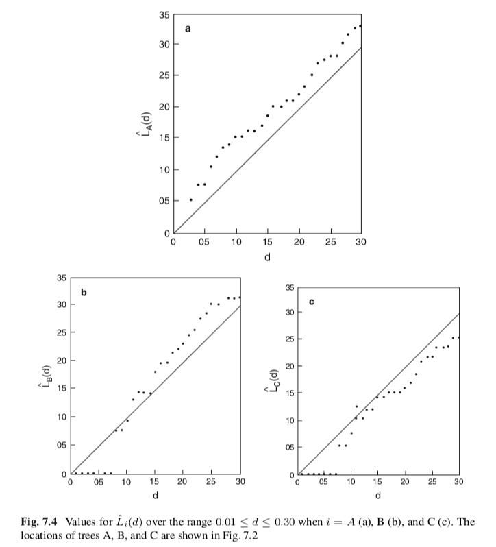
We can see that in plot a, $L(t)$ is above the line with its slope equals to 1, which representing the $L(t)$ of CSR. It implied the cluster was formed. While in plot c, the effect is opposite.
The $L(t)$ can also be plotted with isoline with a given distance ($t$):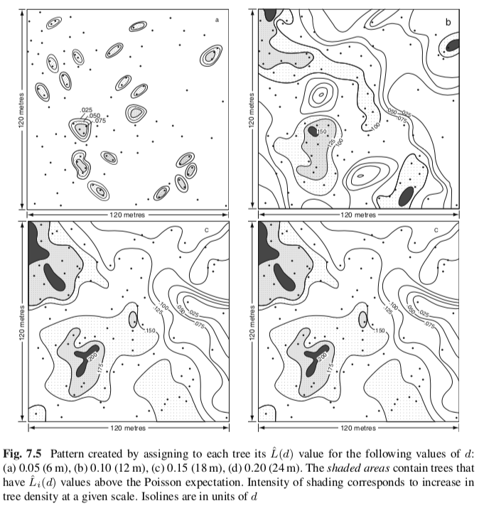
Nanocluster of Membrane Proteins
Bálint published a paper in 2018, using dSTORM microscopy to resolve the nanoclustering of a receptor called natural killer group 2D (NKG2D). One of the challenges using the STROM microscope is to translate thousands, or sometimes millions, of stochastic fluorescent events into meaningful measurements. In this case, they wanted to know the size of nanoclusters and the interactions between them. To achieve that, they extracted the Euclid coordinates, which require:
- performing spatial analysis ($\hat{K}(t)$, $\hat{L}(t)$, and $\hat{H}(t)$)
- generating a density map based on $\hat{H}(t)$,
- thresholding density maps into binary maps
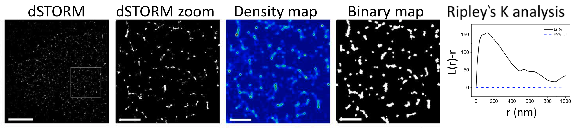
Be aware that under CSR, the $\hat{H}(t)$ value should be 0 (It is $\hat{L}(t) - t$), so $\hat{H}(t)$ reduced when the radius increased.
Implementation
Some software comes with the function of spatial analysis based on Ripley’s K method. I wrote my own Python code for proof of concept, but found that the easiest way to implement is probably using a R package called Spatstat. I will write another post for demonstration.
Reference
Williamson, D. J., Owen, D. M., Rossy, J., Magenau, A., Wehrmann, M., Gooding, J. J., & Gaus, K. (2011). Pre-existing clusters of the adaptor Lat do not participate in early T cell signaling events. Nature Immunology, 12(7), 655–662. http://doi.org/10.1038/ni.2049
Bálint, Š., Lopes, F. B., & Davis, D. M. (2018). A nanoscale reorganization of the IL-15 receptor is triggered by NKG2D in a ligand-dependent manner. Science Signaling, 11(525), eaal3606. http://doi.org/10.1126/scisignal.aal3606
Ripley, B. D. (1977). Modelling spatial patterns (with discussion). JR Statist. Soc. B, 39, 172-212.(1981) Spatial Statistics.
Getis, A. (1984). Interaction Modeling Using Second-Order Analysis. Environment and Planning A, 16(2), 173–183. http://doi.org/10.1068/a160173
Getis, A., Franklin, J. (1987) Second-Order Neighborhood Analysis of Mapped Point Patterns. Ecology 68:473-477. Reprinted with permission of The Ecological Society of America, Washington DC Link to my paper3 database
Getis, A., & Franklin, J. (2008). Second-Order Neighborhood Analysis of Mapped Point Patterns. In Perspectives on Spatial Data Analysis (pp. 93–100). Berlin, Heidelberg: Springer Berlin Heidelberg. http://doi.org/10.1007/978-3-642-01976-0_7
Book & Other Resource
Books for Spatial statistics