3 minutes
Ripley’s K Demo: 01 Point Process Simulation
- Before demonstrating Ripley’s K function ($K(t)$), $L(t)$, and $H(t)$), I have to first simulate two types of point process: 1. Poisson point process and 2. Thomas point process.
- The point process generator is adpated from Connor Johnson’s blog post.
- The default size of point process generator is 20 x 20
- Please visit the code on my GitHub
# denpendency
import os, sys
import scipy.stats
import pandas as pd
import numpy as np
import matplotlib.pyplot as plt
import matplotlib.style
import matplotlib as mpl
import spatialstat.ppsim as ppsim
%load_ext autoreload
%autoreload 2
# define IO dir
path = '.'
opdir = os.path.join(path, 'output')
opdir_csv = os.path.join(opdir, 'csv')
opdir_fig = os.path.join(opdir, 'figure')

if not os.path.exists(opdir):
    os.makedirs(opdir)
if not os.path.exists(opdir_csv):
    os.makedirs(opdir_csv)
if not os.path.exists(opdir_fig):
    os.makedirs(opdir_fig)

print(opdir)
print(opdir_csv)
print(opdir_fig)
./output
./output/csv
./output/figure
Poisson Point Process
- Create Poisson PP by
ppsim.PoissonPP. Please visit the code on my GitHub - export to *.csv
# Set seed
seed = 1219
rate = 1
Dx = 20

# set data range
xmin = 0
xmax = Dx
ymin = 0
ymax = Dx

P_PoissonPP = ppsim.PoissonPP(rt = rate, seed = seed)
# calculate density
P_PoissonPP_density = ppsim.xydensity(P_PoissonPP)

# save to csv
filename = 'P_PoissonPP_' + str(Dx)
outputpath = os.path.join(opdir_csv, filename + '.csv')
df = pd.DataFrame(P_PoissonPP, columns = ['x', 'y'])
df.to_csv(outputpath, index = False)

print("Size of the PoissonPP array: {}".format(P_PoissonPP.shape))
print("Density the PoissonPP array: {}".format(P_PoissonPP_density[0]))
Size of the PoissonPP array: (398, 2)
Density the PoissonPP array: 1.0070902229053578
Thomas Point Process
- Create Thomas PP from given parent points generated from Poison PP
- Create Thomas PP by
ppsim.ThomasPP. Please visit the code on my GitHub - export to *.csv
# Set seed
seed = 1219
rate = 0.1
Dx = 20

# create parent points
P_parent = ppsim.PoissonPP(rt = rate, seed = seed)
print("Size of the P_parent array: {}".format(P_parent.shape))
Size of the P_parent array: (39, 2)
# create children points
sigma = 0.3
mu = 50
P_children, P_parent = ppsim.ThomasPP(rt = rate,
                                sigma = sigma, mu = mu, seed = seed)
# reduce data to region of interest
xmin = 0
xmax = Dx
ymin = 0
ymax = Dx

# crop data and calculate density
P_ThomasPP = ppsim.xyroi(P_children, xmin, xmax, ymin, ymax)
P_ThomasPP_density = ppsim.xydensity(P_ThomasPP)

# save to csv
filename = 'P_ThomasPP_20'
outputpath = os.path.join(opdir_csv, filename + '.csv')
df = pd.DataFrame(P_ThomasPP, columns = ['x', 'y'])
df.to_csv(outputpath, index = False)

print("Size of the ThomasPP array: {}".format(P_ThomasPP.shape))
print("Density the ThomasPP array: {}".format(P_ThomasPP_density[0]))
0 20 0 20
Size of the ThomasPP array: (1898, 2)
Density the ThomasPP array: 5.359077104022789
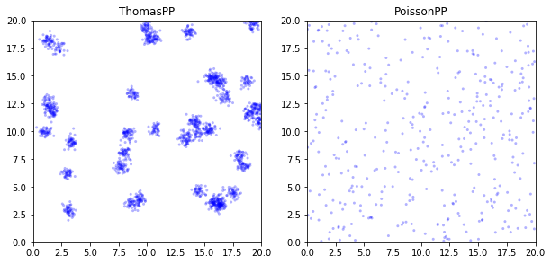
Plot Poisson and Thomas PP
Now having point process we need, we can make plots and show them side-by-side.
# set figure size
plt.figure(figsize= (10, 10))
plotsize_x = 20.0
plotsize_y = 20.0

# subplot 1
plot_1 = plt.subplot(221)
plot_1.scatter(P_children[:, 0], P_children[:, 1],
                color = 'b', edgecolors = 'none', marker = '.', alpha =0.3)
plot_1.set_title('ThomasPP')
plot_1.set_xlim([0,20])
plot_1.set_ylim([0,20])

# subplot 2
plot_2 = plt.subplot(222)
plot_2.scatter(P_PoissonPP[:, 0], P_PoissonPP[:, 1],
                color = 'b', edgecolors = 'none', marker = '.', alpha =0.3)
plot_2.set_title('PoissonPP')
plot_2.set_xlim([0,20])
plot_2.set_ylim([0,20])

# save figure
filename = 'Point_Process_20'
outputpath = os.path.join(opdir_fig, filename + '.png')
plt.savefig(outputpath)

plt.show()
What Next…
In this simulation, it is easy to visually identify the clustering in Thomas Point Process. In the next post, I will demonstrate how to perfrom Ripley’s K test by using our customized code, so we measure the relationship of density and distance.
551 Words
2020-04-18 05:00 -0500
comments powered by Disqus